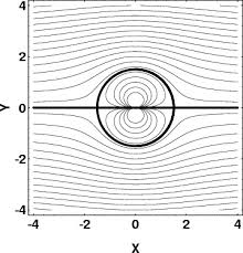
potential flow model [tower wake]: xref:NextGen_Towershadow#powles-empirical-model [Powles]: xref:NextGen_references#Powles_S_R_J_1983 [inverse square root variation]: xref:NextGen_Towershadow#inverse-square-root-variation

Tower Shadow

Tower shadow defines the distortion of the steady-state mean flow field due to the presence of the turbine tower or support structure. Three different models are available: a [potential flow model] for upwind rotors, an empirical [tower wake] model for downwind rotors, and a combined model which is useful if the rotor yaws in and out of the down wind shadow area.

Potential flow model

This model is appropriate for rotors operating up wind of the tower. The longitudinal wind velocity component up wind of the tower \(\bscalar{{V}_0}\) is modified using the assumption of incompressible laminar flow around a cylinder of diameter \(\bscalar{D}=\bscalar{F}\cdot \bscalar{D_T}\) where \(\bscalar{D_T}\) is the tower diameter at the height where the tower shadow is being calculated, and \(\bscalar{F}\) is a tower diameter correction factor supplied by the user.

Potential flow around cylinder — Figure 1: Potential Flow around cylinder

For a point in GL coordinates at a distance \(\bscalar{x}\) in front of the tower centreline and \(\bscalar{y}\) to the side of the wind vector passing through the centreline, the wind speed in the plane perpendicular to the tower axis, \(\bvector{V}\), is given by:

\[ \begin{equation} \bvector{V}=\bscalar{V_0}\bvector{i}+\left(\bscalar{\frac{\left(y^2-x^2\right)}{\left(y^2+x^2\right)^2}}\bvector{i}+\bscalar{\frac{-2xy}{\left(y^2+x^2\right)^2}}\bvector{j}\right)\left(\bscalar{\frac{D}{2}}\right)^2\bscalar{V_0} \end{equation} \]

where, i, and j are the unit vectors in the x and y directions. This is provided that the point is far from the tower top. For the variation close to the tower top see application to multi-member towers and end effects.

Powles empirical model

For rotors operating downwind of the tower, an empirical model is provided, based on the work of [Powles] which uses a cosine bell-shaped tower wake. For a point at a distance \(\bscalar{x}\) behind the tower centreline and \(\bscalar{y}\) to the side of the wind vector passing through the centreline, the wind speed perpendicular to the tower axis, \(\bvector{V}\), is given by:

\[ \begin{equation} \bscalar{V}=\bscalar{\left[1-\Delta(x){\cos}^2{\left(\frac{\pi y}{WD_T}\right)}\right]}\bscalar{V_0} \end{equation} \]

Here \(\bscalar{\Delta(x)}\) is the maximum velocity deficit at the centre of the wake expressed as a fraction of the local wind speed, and \(\bscalar{W}\) is the width of the tower shadow expressed as a proportion of the local tower diameter \(\bscalar{D_T}\). Both \(\Delta(x)\) and \(\bscalar{W}\) are a function of \(\bscalar{x}\), the downwind distance of the point using an [inverse square root variation].

Inverse square root variation

This is the default case, where \(\bscalar{W}\) increases proportionally to the square root of the downwind distance, and the maximum deficit, \(\bscalar{\Delta(x)}\), scales in inverse proportion to the square root of the distance.

\[ \begin{equation} \bscalar{l(x)=\sqrt{\frac{x}{D_Tl_{ref}}}} \end{equation} \]

and,

\[ \begin{equation} \bscalar{W = W l(x)} \end{equation} \]

\[ \begin{equation} \bscalar{\Delta(x)=\frac{\Delta_{max}}{l}} \end{equation} \]

Where \(W\) is the width of the tower input by the user, \(\Delta_{max}\) is the maximum velocity deficit input by the user and \(\bscalar{l_{ref}}\) is the number of times the local tower diameter downwind at which the user-specified values for the wake width and maximum deficit is applicable.

Wake using inverse square variation — Figure 2: Wake (inverse square variation)

No variation

Where there is no downwind variation in wake, the width of the wake and the maximum deficit are constant. Below is pictured the wake when \(\bscalar{W=1.0}\).

Combined model

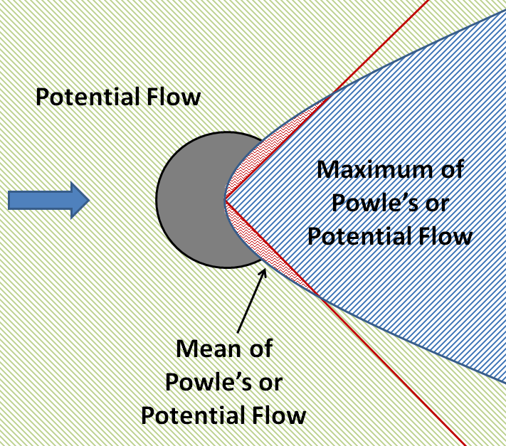
The combined model uses Potential Flow Theory for a majority of the flow-field, but uses a combination of Powle's and Potential Flow in the region where Powle's is active (i.e. within the wake according to whichever downwind variation that the Powle's model is using).

Rearwards of a 45° line, the method which results in the maximum perturbation is used. Forwards of that line, an average of the two methods is used, so long as the Powles' model is in effect.

Application to multi-member towers and end effects

For multi-member towers, the effective wind speed changes due to each member are calculated individually, using the chosen method, and summed. The magnitude of the total change is limited to the magnitude of the original velocity. Both the potential flow and Powles models only modify the components of velocity perpendicular to the member axis.

The effect close to the end of the member varies smoothly for both potential flow and Powles models. For the potential flow model, the member is assumed to be a line source with ends at positions \(\bscalar{p_1}\) and \(\bscalar{p_2}\). Hence, in a coordinate system with the \(\bscalar{z}\) axis pointing along the tower (or member) the resulting velocity is given by:

\[ \begin{equation} \begin{aligned} & \bvector{V}=\bvector{V_0} + \left(\bscalar{B}\bvector{i}+\bscalar{C}\bvector{j}\right)\left(\frac{\bscalar{D}}{\bscalar{2}}\right)^2\bscalar{V_{0xy}}, \\ & \bscalar{B=\frac{\left(z-p_2\right)\left(y^2-x^2\right)}{\left(y^2+x^2\right)^2\left(x^2+y^2+(z-p_2)^2\right)^\frac{1}{2}}+\frac{\left(z-p_2\right)x^2}{\left(y^2+x^2\right)\left(x^2+y^2+(z-p_2)^2\right)^\frac{3}{2}}- \\ & \quad \quad \ \frac{\left(z-p_1\right)\left(y^2-x^2\right)}{\left(y^2+x^2\right)^2\left(x^2+y^2+(z-p_1)^2\right)^\frac{1}{2}}-\frac{\left(z-p_1\right)x^2}{\left(y^2+x^2\right)\left(x^2+y^2+(z-p_1)^2\right)^\frac{3}{2}}}, \\ & \bscalar{C=\frac{-2xy\left(z-p_2\right)}{\left(y^2+x^2\right)^2\left(x^2+y^2+(z-p_2)^2\right)^\frac{1}{2}}-\frac{xy\left(z-p_2\right)}{\left(y^2+x^2\right)\left(x^2+y^2+(z-p_2)^2\right)^\frac{3}{2}}+ \\ & \quad \quad \ \frac{2xy\left(z-p_1\right)}{\left(y^2+x^2\right)^2\left(x^2+y^2+(z-p_1)^2\right)^\frac{1}{2}}+\frac{xy\left(z-p_1\right)}{\left(y^2+x^2\right)\left(x^2+y^2+(z-p_1)^2\right)^\frac{3}{2}}} \end{aligned} \end{equation} \]

where, \(\bscalar{V_{0xy}}\) is the magnitude of the velocity in the \(\bscalar{x-y}\) plane, \(i\) and \(j\) are the unit vectors in the \(x\) and \(y\) directions.

For the Powles model, the end effects are taken account of by simplifying it to a diffusion equation. For line source in the diffusion equation, the fall off at the ends of the source is proportional to the error function:

\[ \begin{equation} \bscalar{A=\left(1-\Delta{\cos}^2{\left(\frac{\pi y}{WD_T}\right)}\right)\left(erf\left(\frac{2\left(z-p_2\right)}{\sqrt{WD_T}}\right)-erf\left(\frac{2\left(z-p_1\right)}{\sqrt{WD_T}}\right)\right)} \end{equation} \]