Plot a turbine in 3D using Python
The samples presented in this article are a series of functions and scripts that will plot a turbine assembly and it's components in 3D. The component scripts will work with any of the following components:
- Tower:
plot_tower.py - Hub:
plot_hub.py - Drivetrain and Nacelle:
plot_drivetrain_and_nacelle.py - Blade:
plot_blade.py
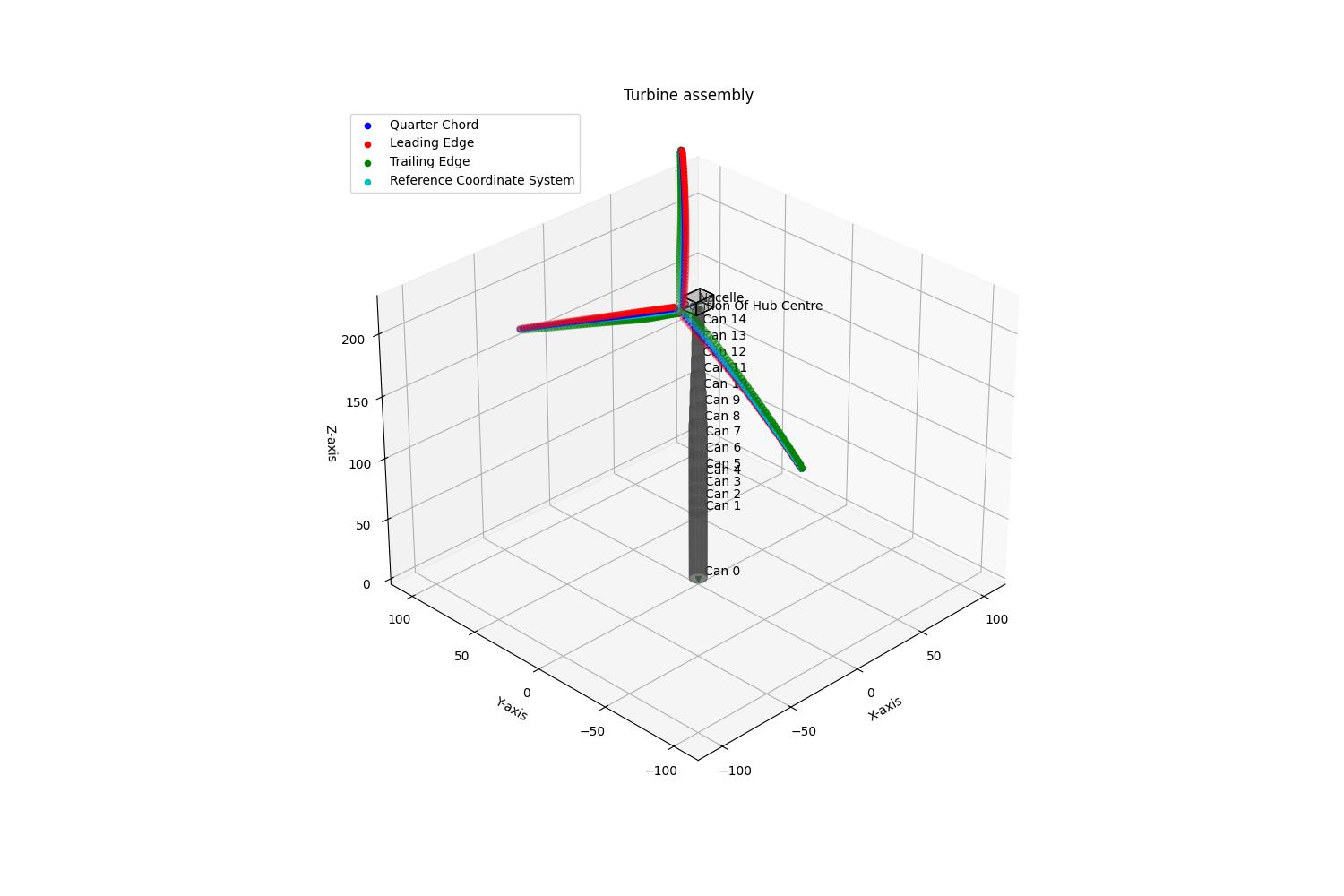
The final sample connects (plot_assembly.py) all the components and plots in a full 3D turbine assembly.
The scripts in their supplied form plot the IEA 15MW turbine (NG_IEA_15_Onshore_SteadyOP.json). They can be used with other turbines, but they need to have the same components and the same structure. For different structures and extra components the user will have to change the files themselves.
Prerequisites
- Latest version of Bladed Next Gen and Samples installed including the Bladed Python packages.
- Licence for Bladed Next Gen (request a licence).
- Python 3.9 to 3.12 installed.
What you will learn
- Identifying the JSON input file geometry properties and what they mean in a 3D space.
How to use this tutorial
To use this tutorial it is advised to download the samples. The package contains all required content to complete this tutorial.
Make sure to check the Get started article on how to setup your machine for the tutorials.
Switch to the samples folder and run each of the Python scripts described in this article.
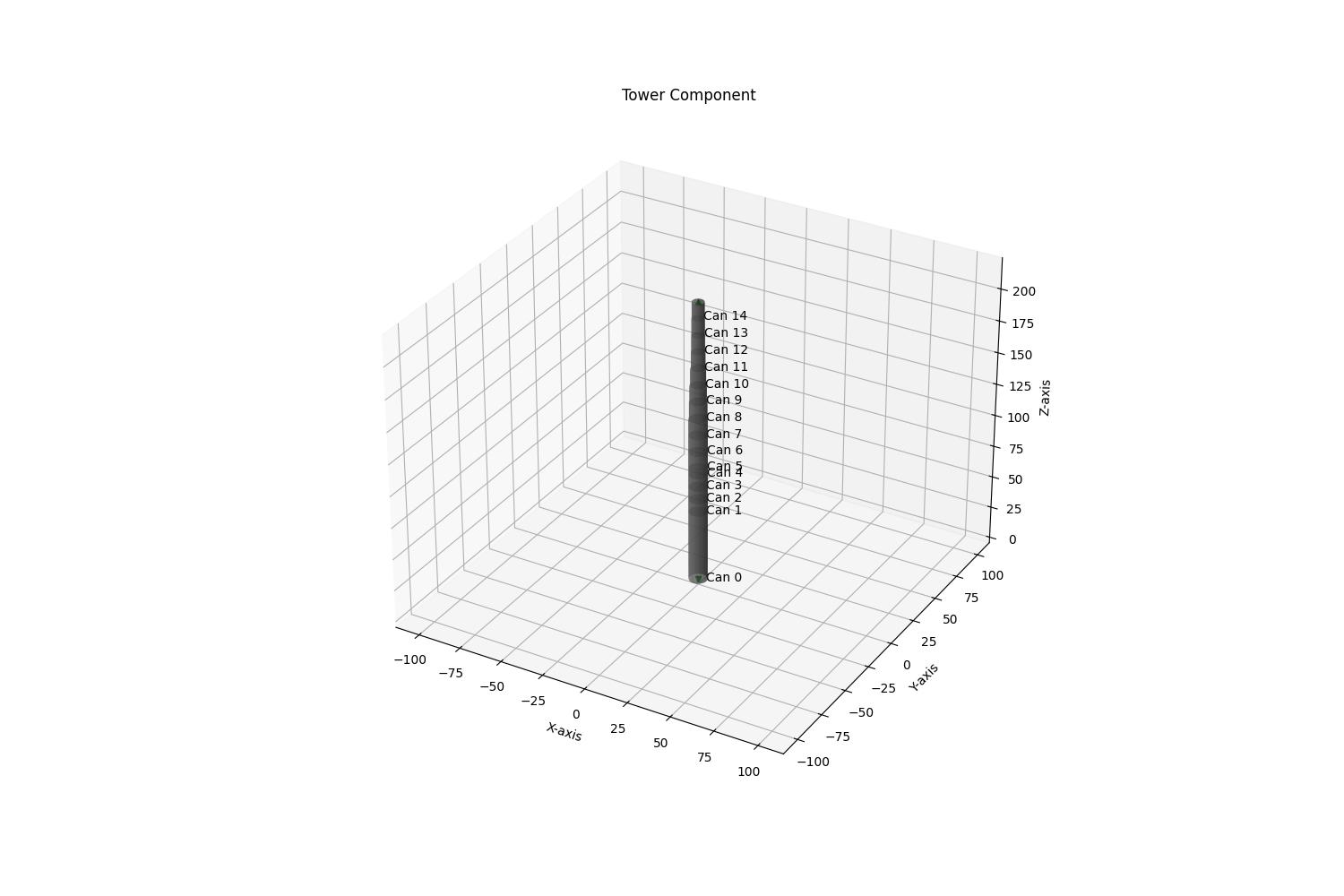
Plot a tower
"""
plot_tower.py

This example script demonstrates how to plot the Tower component of the provided NG_IEA_15_Onshore_SteadyOP turbine model.
It showcases how to extract input data and visualize it using 3D plots.

Please note that this script is specific to the NG_IEA_15_Onshore_SteadyOP model and may not be compatible with other turbine models.

Requirements:
- tower_plot.py
- dnv_bladed_models (imported as models)
- numpy
- matplotlib

Usage:
1. Ensure that the required components (tower_plot.py, dnv_bladed_models) are available.
2. Make sure the required files and the NG_IEA_15_Onshore_SteadyOP.json are in the same folder.
3. Run the script to visualize the Tower component in a 3D plot.
"""

import os
import dnv_bladed_models as models
import matplotlib.pyplot as plt
import numpy as np

def plot_tower(figure_axis, tower):
    # Plots a tower structure using 3D surface plots for each can section.

    # Extract information from the Tower object
    can_list = tower.Cans
    first_can = True
    tower_height = 0

    # Iterate through each can in the list
    for i_can, can in enumerate(can_list):
        can_height = can.CanHeight
        # Calculate starting point and previous height
        if first_can:
            first_can = False
            can_starting_point = 0
            previous_height = can_height
        else:
            can_starting_point = previous_height
            previous_height = can_starting_point + can_height

        # Calculate base and top radii
        base_outer_radius = can.BaseSection.OutsideDiameter / 2
        base_inner_radius = can.BaseSection.OutsideDiameter / 2 - can_list[0].BaseSection.WallThickness

        if hasattr(can_list[0], 'TopSection'):
            if not can_list[0].TopSection is None:
                top_outer_radius = can.TopSection.OutsideDiameter / 2
                top_inner_radius = can.TopSection.OutsideDiameter / 2 - can_list[0].TopSection.WallThickness
            else:
                top_outer_radius = base_outer_radius
                top_inner_radius = base_inner_radius
        else:
            top_outer_radius = base_outer_radius
            top_inner_radius = base_inner_radius

        tower_height = tower_height + can.CanHeight

        # Plot surfaces for outer and inner radii
        x_grid, y_grid, z_grid = can_surface(base_outer_radius, top_outer_radius, can_starting_point, can_height)

        figure_axis.plot_surface(x_grid, y_grid, z_grid, alpha=0.5, color='grey')
        figure_axis.text(x_grid[0][0], y_grid[0][0], z_grid[0][0], 'Can '+str(i_can))

        x_grid, y_grid, z_grid = can_surface( base_inner_radius, top_inner_radius, can_starting_point, can_height)

        figure_axis.plot_surface(x_grid, y_grid, z_grid, alpha=0.5, color='k')

    # Set plot limits
    x_max = max(x_grid.max(), y_grid.max(), z_grid.max())
    plt.xlim([-x_max / 2, x_max / 2])
    plt.ylim([-x_max / 2, x_max / 2])
    figure_axis.set_zlim(0, x_max)

    # Plot assembly nodes
    figure_axis.scatter3D(0, 0, 0, marker='v', color="green")
    assembly_node = np.array([0, 0, tower_height])
    figure_axis.scatter3D(assembly_node[0], assembly_node[1], assembly_node[2], marker='^', color="green")

    return assembly_node


def can_surface(base_radius, top_radius, can_starting_point, can_height):
    # Generates a 3D surface representation of a truncated cone (can) using parametric equations

    # Create an array of z values along the height of the can
    z = np.linspace(can_starting_point, can_starting_point+can_height, 5)

    # Create an array of theta values (angle around the z-axis)
    theta = np.linspace(0, 2*np.pi, 50)

    # Create a grid of theta and z values
    theta_grid, z_grid = np.meshgrid(theta, z)

    # Calculate the varying radius along the height
    radius = base_radius + (top_radius - base_radius) * z_grid / can_height

    # Calculate x and y coordinates using polar coordinates
    x_grid = radius*np.cos(theta_grid)
    y_grid = radius*np.sin(theta_grid)

    return x_grid, y_grid, z_grid


if __name__ == "__main__":

    # Specify required folders, relative to this script
    examples_models_path = os.path.dirname(__file__)

    # read in a full analysis from file
    analysis_model_file_path = os.path.join(examples_models_path, 'NG_IEA_15_Onshore_SteadyOP.json')

    # Extract the components of the project file
    Components = models.BladedAnalysis.from_file(analysis_model_file_path).ComponentDefinitions

    # Figure settings
    fig, figure_axis = plt.subplots(subplot_kw={"projection": "3d"}, figsize=(15, 10))
    figure_axis.set(xlabel='X-axis', ylabel='Y-axis', zlabel='Z-axis')
    figure_axis.set_title("Tower Component")

    # Plots the tower
    plot_tower(figure_axis, Components['IEA15Tower'])

    plt.show()
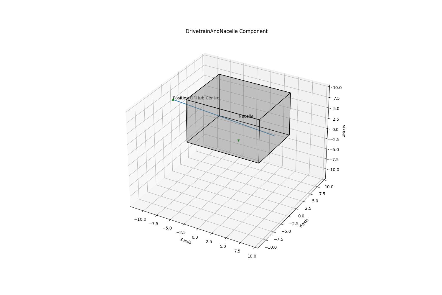
Plot a nacelle and drivetrain
"""
plot_drivetrain_and_nacelle.py

This example script demonstrates how to plot the DrivetrainAndNacelle component of the provided NG_IEA_15_Onshore_SteadyOP turbine model.
It showcases how to extract input data and visualize it using 3D plots.

Please note that this script is specific to the NG_IEA_15_Onshore_SteadyOP model and may not be compatible with other turbine models.

Requirements:
- drivetrain_and_nacelle_plot.py
- dnv_bladed_models (imported as models)
- numpy
- scipy
- matplotlib

Usage:
1. Ensure that the required components (drivetrain_and_nacelle_plot.py, dnv_bladed_models) are available.
2. Make sure the required files and the NG_IEA_15_Onshore_SteadyOP.json are in the same folder.
3. Run the script to visualize the DrivetrainAndNacelle component in a 3D plot.
"""

import os
import dnv_bladed_models as models
import matplotlib.pyplot as plt
import numpy as np
from scipy.spatial.transform import Rotation as R
from mpl_toolkits.mplot3d.art3d import Poly3DCollection

def create_box_points_and_faces(centre, length, width, height, initial_coordinates):
    # Creates points and faces for a 3D box (cuboid) given its center, dimensions, and initial coordinates.

    half_length = length / 2
    half_width = width / 2
    half_height = height / 2

    # Define the 8 corner points of the box
    points = np.array([
        [centre[0] - half_length, centre[1] - half_width, centre[2] - half_height],
        [centre[0] + half_length, centre[1] - half_width, centre[2] - half_height],
        [centre[0] + half_length, centre[1] + half_width, centre[2] - half_height],
        [centre[0] - half_length, centre[1] + half_width, centre[2] - half_height],
        [centre[0] - half_length, centre[1] - half_width, centre[2] + half_height],
        [centre[0] + half_length, centre[1] - half_width, centre[2] + half_height],
        [centre[0] + half_length, centre[1] + half_width, centre[2] + half_height],
        [centre[0] - half_length, centre[1] + half_width, centre[2] + half_height]
    ]) + initial_coordinates

    # Define the faces of the box (each face as a list of points)
    faces = [[points[0], points[1], points[2], points[3]],
             [points[4], points[5], points[6], points[7]],
             [points[0], points[1], points[5], points[4]],
             [points[2], points[3], points[7], points[6]],
             [points[1], points[2], points[6], points[5]],
             [points[4], points[7], points[3], points[0]]]

    return points, faces


def plot_nacelle(figure_axis, drivetrain_and_nacelle, initial_coordinates=np.array([0.0, 0.0, 0.0])):
    # PLots the nacelle assembly in 3D space

    # Specify dimensions (width, length, height)
    width = drivetrain_and_nacelle.NacelleCover.Width
    length = drivetrain_and_nacelle.NacelleCover.Length
    height = drivetrain_and_nacelle.NacelleCover.Height

    # Specify the centre point (x, y, z). Assumes the geometric centre coincides with the centre of pressure.
    centre = (drivetrain_and_nacelle.NacelleCover.CentreOfPressure.X,
              drivetrain_and_nacelle.NacelleCover.CentreOfPressure.Y,
              drivetrain_and_nacelle.NacelleCover.CentreOfPressure.Z)  # centre position (x, y, z)

    # Specify hub assembly point and direction
    hub_assembly_point = np.zeros(3)
    hub_assembly_point[0] = - drivetrain_and_nacelle.PositionOfHubCentre.Overhang
    hub_assembly_point[1] = drivetrain_and_nacelle.PositionOfHubCentre.SideOffset
    hub_assembly_point[2] = drivetrain_and_nacelle.PositionOfHubCentre.HeightOffset

    # Tilt rotation matrix
    hub_assembly_tilt = R.from_euler('y', drivetrain_and_nacelle.PositionOfHubCentre.RotorTilt).as_matrix()

    # Compute the eight corner points (vertices) and faces
    points, faces = create_box_points_and_faces(centre, length, width, height, initial_coordinates)

    # Plot the parallelepiped
    figure_axis.scatter3D(*points.T, color='red', alpha=0)  # Plot vertices

    # Plot the faces
    figure_axis.add_collection3d(Poly3DCollection(faces, facecolors='grey', linewidths=1, edgecolors='black', alpha=0.25))

    # Plot previous assembly point
    figure_axis.scatter3D(*initial_coordinates, color='g', marker='v')

    # Rotate hub pitch:
    shaft_unit_vector = hub_assembly_tilt.dot(np.array([1.0, 0.0, 0.0]))

    # Start location of the low speed shaft
    shaft_start = np.array([0.0, 0.0, 0.0])
    shaft_start[0] = hub_assembly_point[0] + (length/2-hub_assembly_point[0]) * shaft_unit_vector[0]
    shaft_start[1] = hub_assembly_point[1]
    shaft_start[2] = hub_assembly_point[2] + (length/2-hub_assembly_point[0]) * shaft_unit_vector[2]

    # Rotate as to horizontal of nacelle:
    shaft_start = shaft_start + initial_coordinates

    # Rotate assembly
    hub_assembly_point = hub_assembly_point + initial_coordinates

    # Plot next assembly point
    figure_axis.scatter3D(hub_assembly_point[0], hub_assembly_point[1], hub_assembly_point[2], color='g', marker='^')

    figure_axis.text(hub_assembly_point[0], hub_assembly_point[1], hub_assembly_point[2], 'Position Of Hub Centre')

    # Nacelle mid point
    midpoint = np.average(points, axis=0)

    figure_axis.text(midpoint[0], midpoint[1], midpoint[2], 'Nacelle')

    # Plot shaft
    figure_axis.plot([hub_assembly_point[0], shaft_start[0]], [hub_assembly_point[1], shaft_start[1]], zs=[hub_assembly_point[2], shaft_start[2]])

    plt.xlim([min(hub_assembly_point[0], initial_coordinates[1]-width/2, initial_coordinates[2]-height),
             max(initial_coordinates[0]+length/2, initial_coordinates[1]+width/2, initial_coordinates[2]+height)])
    plt.ylim([min(hub_assembly_point[0], initial_coordinates[1]-width/2, initial_coordinates[2]-height),
             max(initial_coordinates[0]+length/2, initial_coordinates[1]+width/2, initial_coordinates[2]+height)])
    figure_axis.set_zlim(min(hub_assembly_point[0], initial_coordinates[1]-width/2, initial_coordinates[2]-height), max(
        initial_coordinates[0]+length/2, initial_coordinates[1]+width/2, initial_coordinates[2]+height))

    return hub_assembly_point, hub_assembly_tilt


if __name__ == "__main__":

    # Specify required folders, relative to this script
    examples_models_path = os.path.dirname(__file__)

    # Read in a full analysis from file
    analysis_model_file_path = os.path.join(examples_models_path, 'NG_IEA_15_Onshore_SteadyOP.json')

    # Extract the components of the project file
    Components = models.BladedAnalysis.from_file(analysis_model_file_path).ComponentDefinitions

    # Figure settings
    fig, figure_axis = plt.subplots(subplot_kw={"projection": "3d"}, figsize=(15, 10))
    figure_axis.set(xlabel='X-axis', ylabel='Y-axis', zlabel='Z-axis')
    figure_axis.set_title("DrivetrainAndNacelle Component")

    # Plots the nacelle and drivetrain low speed shaft
    plot_nacelle(figure_axis, Components['IEA15DrivetrainAndNacelle'])

    plt.show()
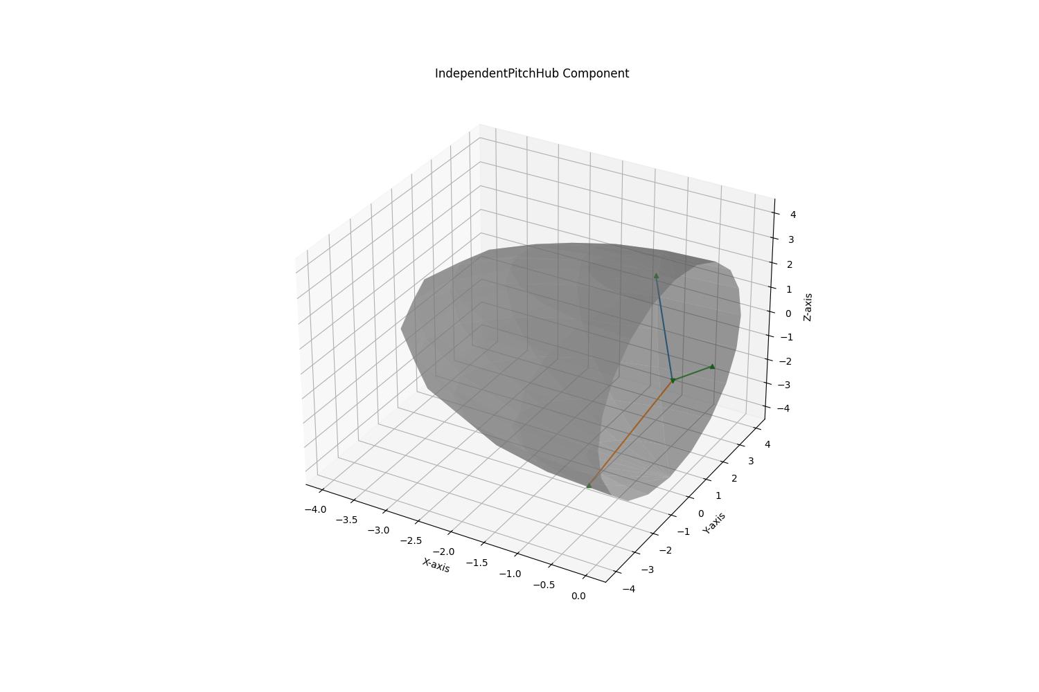
Plot a blade hub
"""
plot_hub.py

This example script demonstrates how to plot the Hub component of the provided NG_IEA_15_Onshore_SteadyOP turbine model.
It showcases how to extract input data and visualize it using 3D plots.

Please note that this script is specific to the NG_IEA_15_Onshore_SteadyOP model and may not be compatible with other turbine models.

Requirements:
- hub_plot.py
- dnv_bladed_models (imported as models)
- numpy
- scipy
- matplotlib

Usage:
1. Ensure that the required components (hub_plot.py, dnv_bladed_models) are available.
2. Make sure the required files and the NG_IEA_15_Onshore_SteadyOP.json are in the same folder.
3. Run the script to visualize the Hub component in a 3D plot.
"""

import os
import dnv_bladed_models as models
import matplotlib.pyplot as plt
import numpy as np
from scipy.spatial.transform import Rotation as R

def plot_hub(figure_axis, hub, rotor_tilt=np.eye(3), initial_coordinates=np.array([0.0, 0.0, 0.0])):
    # Plots the hub and calculates the blade mounting points

    # Radius of the hub
    hub_radius = hub.Spinner.Diameter/2

    # Plot the hub as a sphere
    plot_half_sphere(figure_axis, hub_radius, initial_coordinates)

    blade_rotations = []
    blade_starting_points = []
    azimuth_step = 2*np.pi/hub.NumberOfBlades

    for i in range(0, hub.NumberOfBlades):
        # Calculates the blade mounting rotations, direction and the starting points

        # Calculate the rotation matrix to rotate due to different azimuth positions and coning rotation
        rot_azimuth = R.from_euler('x', azimuth_step*i).as_matrix()
        rot_cone = R.from_euler('y', - hub.MountingPoints.ConingAngle).as_matrix()

        # Final rotation matrix due to tilt, azimuth and coning angle
        blade_rotations.append(rotor_tilt.dot(rot_azimuth.dot(rot_cone)))

        blade_directions = blade_rotations[i].dot(np.array([0.0, 0.0, 1.0]))

        blade_starting_points.append(initial_coordinates + blade_directions * hub.MountingPoints.RadiusOfBladeConnection)

        # Plot blade connections
        figure_axis.plot([initial_coordinates[0], blade_starting_points[i][0]], [
                        initial_coordinates[1], blade_starting_points[i][1]], zs=[initial_coordinates[2], blade_starting_points[i][2]])

        # Plot blade starting points
        figure_axis.scatter3D(blade_starting_points[i][0], blade_starting_points[i][1], blade_starting_points[i][2], color='g', marker='^')

    # Plot hub center
    figure_axis.scatter3D(initial_coordinates[0], initial_coordinates[1], initial_coordinates[2], color='g', marker='v')

    return blade_starting_points, blade_rotations


def plot_half_sphere(figure_axis, radius, initial_coordinates):

    # Define the number of steps
    step = np.pi/10

    # Define the co-ordinates of points in the sphere
    phi = np.arange(0 , np.pi + step, step) # Only half of a shpere
    theta = np.arange(np.pi / 2, np.pi * 1.5 + step, step)
    phi, theta = np.meshgrid(phi, theta)

    # Convert spherical coordinates to cartesian coordinates
    x = radius * np.sin(phi) * np.cos(theta) + initial_coordinates[0]
    y = radius * np.sin(phi) * np.sin(theta) + initial_coordinates[1]
    z = radius * np.cos(phi) + initial_coordinates[2]

    # Create a 3D plot
    figure_axis.plot_surface(x, y, z, color='grey', alpha=0.5)

if __name__ == "__main__":

    # Specify required folders, relative to this script
    examples_models_path = os.path.dirname(__file__)

    # Read in a full analysis from file
    analysis_model_file_path = os.path.join(examples_models_path, 'NG_IEA_15_Onshore_SteadyOP.json')

    # Extract the components of the project file
    Components = models.BladedAnalysis.from_file(analysis_model_file_path).ComponentDefinitions

    # Figure settings
    fig, figure_axis = plt.subplots(subplot_kw={"projection": "3d"}, figsize=(15, 10))
    figure_axis.set(xlabel='X-axis', ylabel='Y-axis', zlabel='Z-axis')
    figure_axis.set_title("IndependentPitchHub Component")

    plot_hub(figure_axis, Components['IEA15Hub'])

    plt.show()
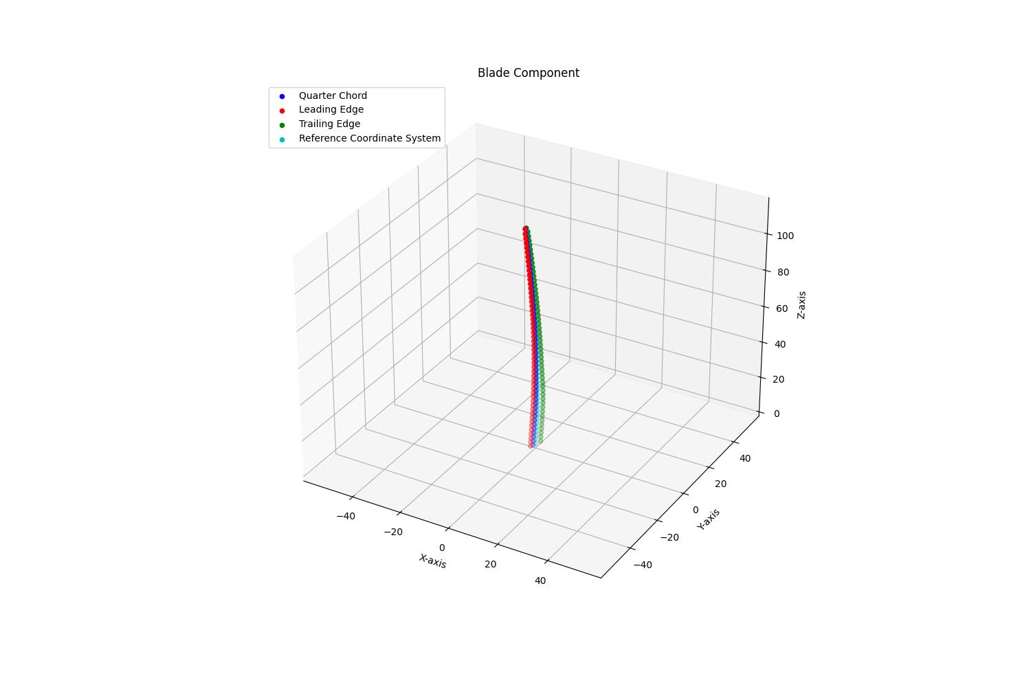
Plot a blade
"""
plot_blade.py

This example script demonstrates how to plot the Blade component of the provided NG_IEA_15_Onshore_SteadyOP turbine model.
It showcases how to extract input data and visualize it using 3D plots.

Please note that this script is specific to the NG_IEA_15_Onshore_SteadyOP model and may not be compatible with other turbine models.

Requirements:
- blade_plot.py
- dnv_bladed_models (imported as models)
- numpy
- scipy

Usage:
1. Ensure that the required components (blade_plot.py, dnv_bladed_models) are available.
2. Make sure the required files and the NG_IEA_15_Onshore_SteadyOP.json are in the same folder.
3. Run the script to visualize the Blade component in a 3D plot.
"""

import os
import numpy as np
import matplotlib.pyplot as plt
import dnv_bladed_models as models
from scipy.spatial.transform import Rotation as R

def plot_blade(figure_axis, blade, initial_coordinates=np.array([0, 0, 0]), blade_rotations=np.eye(3)):
    # Plots the blade given the blade data, initial coordinates and blade mounting angles
    # Transformations are based on the theory presented in the Bladed Next Gen Online Documentation: "Blade Coordinate Systems Theory"

    reference_systems = np.empty((0, 3))
    leading_edges = np.empty((0, 3))
    trailing_edges = np.empty((0, 3))
    quarter_chords = np.empty((0, 3))

    for blade_section in blade.SectionDefinitions:
        # Extract relevant data from blade section
        coordinate_system = blade_section.AxesAndCoordinateSystems
        blade_reference_axis = coordinate_system.ReferenceCoordinateSystem
        blade_aerodynamic_properties = blade_section.AerodynamicProperties
        blade_quarter_chord_axis = coordinate_system.QuarterChordCoordinateSystem

        # Extracts the unit vectors of the reference coordinate system
        unit_z_axis = np.array([blade_reference_axis.ZAxis.X, blade_reference_axis.ZAxis.Y, blade_reference_axis.ZAxis.Z])
        unit_y_axis = np.array([blade_reference_axis.YAxis.X, blade_reference_axis.YAxis.Y, blade_reference_axis.YAxis.Z])
        unit_x_axis = (np.cross(unit_y_axis, unit_z_axis)) / np.linalg.norm(np.cross(unit_y_axis, unit_z_axis))

        # Extract origin and rotation matrix from the blade root cordinate system to the reference coordinate system
        o_root_ref = np.array([blade_reference_axis.Origin.X, blade_reference_axis.Origin.Y, blade_reference_axis.Origin.Z])
        rotation_root_ref = np.column_stack((unit_x_axis, unit_y_axis, unit_z_axis))

        # Extract origin and rotation matrix from the blade reference cordinate system to the quarter chord coordinate system
        rotation_ref_quarter = R.from_euler('z', blade_quarter_chord_axis.RotationAboutReferenceZ).as_matrix()
        o_ref_quarter = np.array([blade_quarter_chord_axis.OffsetInReferenceX, blade_quarter_chord_axis.OffsetInReferenceY, 0.0])

        # Combines them into a rotation and translation from the root coordinate system to the quarter chord coordinate system
        rotation_root_quarter = rotation_root_ref.dot(rotation_ref_quarter)
        o_root_quarter = o_root_ref + rotation_root_ref.dot(o_ref_quarter)

        # Creates the transformation matrix for the QuarterChordCoordinateSystem
        f_qc = np.column_stack((rotation_root_quarter, o_root_quarter))
        f_qc = np.vstack((f_qc, np.array([0, 0, 0, 1])))

        # Uses the transformation matrix to calculate the location of the leading and trailing edge
        leading_edge_location = f_qc.dot(np.array([0, -0.25*blade_aerodynamic_properties.Chord, 0, 1]))[0:3]
        trailing_edge_location = f_qc.dot(np.array([0, 0.75*blade_aerodynamic_properties.Chord, 0, 1]))[0:3]
        quarter_chord_location = f_qc[0:3, 3]

        # Rotates the locations to account for the different azimuth positions and adds the initial positions to get them into global coordinates
        quarter_chord_location = blade_rotations.dot(quarter_chord_location) + initial_coordinates
        leading_edge_location = blade_rotations.dot(leading_edge_location) + initial_coordinates
        trailing_edge_location = blade_rotations.dot(trailing_edge_location) + initial_coordinates
        reference_system_location = blade_rotations.dot(o_root_ref) + initial_coordinates

        quarter_chords = np.vstack((quarter_chords, quarter_chord_location))
        leading_edges = np.vstack((leading_edges, leading_edge_location))
        trailing_edges = np.vstack((trailing_edges, trailing_edge_location))
        reference_systems = np.vstack((reference_systems, reference_system_location))

    # Plots the quarter chord location, trailing edge and the leading edge
    figure_axis.scatter3D(quarter_chords[:, 0], quarter_chords[:, 1], quarter_chords[:, 2], color='b', label='Quarter Chord')
    figure_axis.scatter3D(leading_edges[:, 0], leading_edges[:, 1], leading_edges[:, 2], color='r', label='Leading Edge')
    figure_axis.scatter3D(trailing_edges[:, 0], trailing_edges[:, 1], trailing_edges[:, 2], color='g', label='Trailing Edge')
    figure_axis.scatter3D(reference_systems[:, 0], reference_systems[:, 1], reference_systems[:, 2], color='c', label='Reference Coordinate System')

    # Update maximum coordinates for plot limits
    maximum = np.max(np.concatenate((quarter_chords, leading_edges, trailing_edges)))
    plt.xlim([-maximum/2, maximum/2])
    plt.ylim([-maximum/2, maximum/2])
    figure_axis.set_zlim(0, maximum)


if __name__ == "__main__":

    # Specify required folders, relative to this script
    examples_models_path = os.path.dirname(__file__)

    # Read in a full analysis from file
    analysis_model_file_path = os.path.join(examples_models_path, 'NG_IEA_15_Onshore_SteadyOP.json')

    # Extract the components of the project file
    Components = models.BladedAnalysis.from_file(analysis_model_file_path).ComponentDefinitions

    # Figure settings
    fig, figure_axis = plt.subplots(subplot_kw={"projection": "3d"}, figsize=(15, 10))
    figure_axis.set(xlabel='X-axis', ylabel='Y-axis', zlabel='Z-axis')
    figure_axis.set_title("Blade Component")

    # Plots the blade
    plot_blade(figure_axis, Components['IEA15Blade'])
    figure_axis.legend(loc = 'upper left')

    plt.show()
Plot a turbine assembly
"""
plot_assembly.py

This example script demonstrates how to plot various components of the provided NG_IEA_15_Onshore_SteadyOP turbine model.
It showcases how to extract input data and visualize it using 3D plots.

Please note that this script is specific to the NG_IEA_15_Onshore_SteadyOP model and may not be compatible with other turbine models.

Requirements:
- blade_plot.py
- dnv_bladed_models (imported as models)
- drivetrain_and_nacelle_plot.py
- hub_plot.py
- tower_plot.py

Usage:
1. Ensure that the required components (blade_plot.py, dnv_bladed_models, drivetrain_and_nacelle_plot.py, hub_plot.py, tower_plot.py) are available.
2. Make sure the required files and the NG_IEA_15_Onshore_SteadyOP.json are in the same folder.
3. Run the script to visualize the turbine components in a 3D plot.
"""

import os
import matplotlib.pyplot as plt
import dnv_bladed_models as models
from plot_blade import plot_blade
from plot_drivetrain_and_nacelle import plot_nacelle
from plot_hub import plot_hub
from plot_tower import plot_tower

if __name__ == "__main__":

    # Specify required folders, relative to this script
    examples_models_path = os.path.dirname(__file__)

    # Read in a full analysis from file
    analysis_model_file_path = os.path.join(examples_models_path, 'NG_IEA_15_Onshore_SteadyOP.json')

    # Extract the components of the project file
    Components = models.BladedAnalysis.from_file(analysis_model_file_path).ComponentDefinitions

    # Figure settings
    fig, figure_axis = plt.subplots(subplot_kw={"projection": "3d"}, figsize=(15, 10))
    figure_axis.set(xlabel='X-axis', ylabel='Y-axis', zlabel='Z-axis')
    figure_axis.set_title("Turbine assembly")
    figure_axis.view_init(elev=30, azim=225)  # Change the viewing angle

    # Utilising the tree-like structure of the Bladed Next Gen turbine assembly to plot the Tower and output the assembly node position for the DrivetrainAndNacelle
    assembly_node = plot_tower(figure_axis, Components['IEA15Tower'])

    # Plot the Nacelle and outputs the assembly node position for the Hub
    assembly_node, rotor_tilt = plot_nacelle(figure_axis, Components['IEA15DrivetrainAndNacelle'], assembly_node)

    # Plot the Hub and outputs the blade mounting points and mounting angles
    blade_starting_points, blade_rotations = plot_hub(figure_axis, Components['IEA15Hub'], rotor_tilt, assembly_node)

    # Plot the Blades
    for i, blade_start_point in enumerate(blade_starting_points):
        plot_blade(figure_axis, Components['IEA15Blade'], blade_start_point, blade_rotations=blade_rotations[i])

    # Only show the legends for the blade AxesAndCoordinateSystems
    handles, labels = plt.gca().get_legend_handles_labels()
    plt.legend(handles[:4], labels[:4], loc = 'upper left')

    plt.show()
